Preceptrons
Table of Contents
Preceptrons - a simple neural network for classfaction
In 1958,Frank Rosenblatt introduced the perceptron, as a simple neural network. The perceptron is a single neuron that takes a set of binary inputs and produces a single output. The output is determined by a weighted sum of the inputs. The weights are real numbers that are messure the importance of each input.
$$ \begin{align} output = \sum_{i=0}^{m}w_i.x_i \end{align} $$
Now the output is a binary value, so to get the value of the output we need to applay the sum of the output to some threshold. The threshold is a real number that determines the value of the output. The output is 1 if the weighted sum is greater than the threshold, and 0 otherwise. $$ \begin{align} output = \begin{cases} \text{1} & \text{if } \sum_{i}w_i.x_i > \text{trheshold}, \ 0 & \text{otherwise.} \end{cases} \end{align} $$
Now when we look at the algebraic representation (2), we can make some aditional simplifications. First the sum can be written as a dot product. $$ \begin{align} output = \begin{cases} \text{1} & \text{if } w^T.x > \text{trheshold}, \ 0 & \text{otherwise.} \end{cases} \end{align} $$
and we can move the threshold to the right side of the equation. $$ \begin{align} output = \begin{cases} \text{1} & \text{if } w^T.x - \text{trheshold} > 0, \ 0 & \text{otherwise.} \end{cases} \end{align} $$
the -threshold in the ML terms is the bias, so we will replace it with a b, you can define the bias as a real number that measure how it easy to output 1, or in more ML terminology, how it easy to fire the neuron.
$$
\begin{align}
\text{b = -threshold} \
\end{align}
$$
$$ \begin{align} output = \begin{cases} 1 & \text{if } w^T.x + b > 0, \ 0 & \text{otherwise.} \end{cases} \end{align} $$
If the bias is large positive, the perceptron almost always outputs 1, because the bias pushes the weighted sum above zero. If the bias is large negative, the perceptron almost always outputs 0, because the bias pushes the weighted sum below zero.
-
A positive bias makes the perceptron easier to activate (the threshold is lower).
-
A negative bias makes the perceptron harder to activate (the threshold is higher).
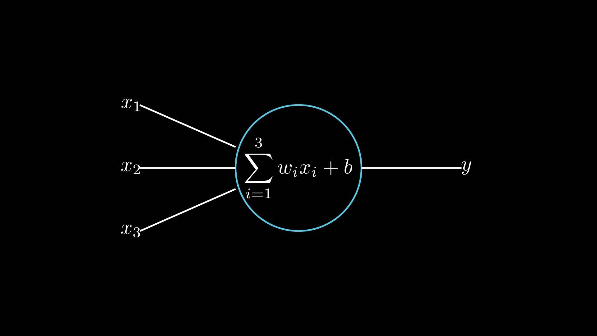
Suppose we have a perceptron with 2 layers, the first layer take 3 inputs $x_1$,$x_2$,and $x_3$, and with there respective weights $w_1$, $w_2$, and $w_3$. And overall biase $b$ the product of the weights and the inputs is $w^T.x + b$. This output from the first layer is the input for the second layer. That what we call the feedforward pass. Such networks are called feedforward neural networks. This means there are no loops in the network - information is always fed forward, never fed back.
Where $z$: $$ \begin{align} z = w^T.x + b \end{align} $$
Sigmoid activation function
The perceptron is a linear function, so the output is always either 0 or 1, but we can use a non-linear function to make the output continuous. The sigmoid function is a good choice because it is smooth and has a range between 0 and 1. $$ \begin{align} \sigma(z) = \frac{1}{1 + e^{-z}} \end{align} $$ There are many other non-linear functions that can be used as activation functions, but the sigmoid function is the most commonly used.
In mathematics what we are really interseted in is the shape of the function, the sigmoid function is a smooth curve that starts at 0 and ends at 1.

The smoothness of sigmoid means that small changes in the weights and in the bias will produce a small change in the output from the neuron.
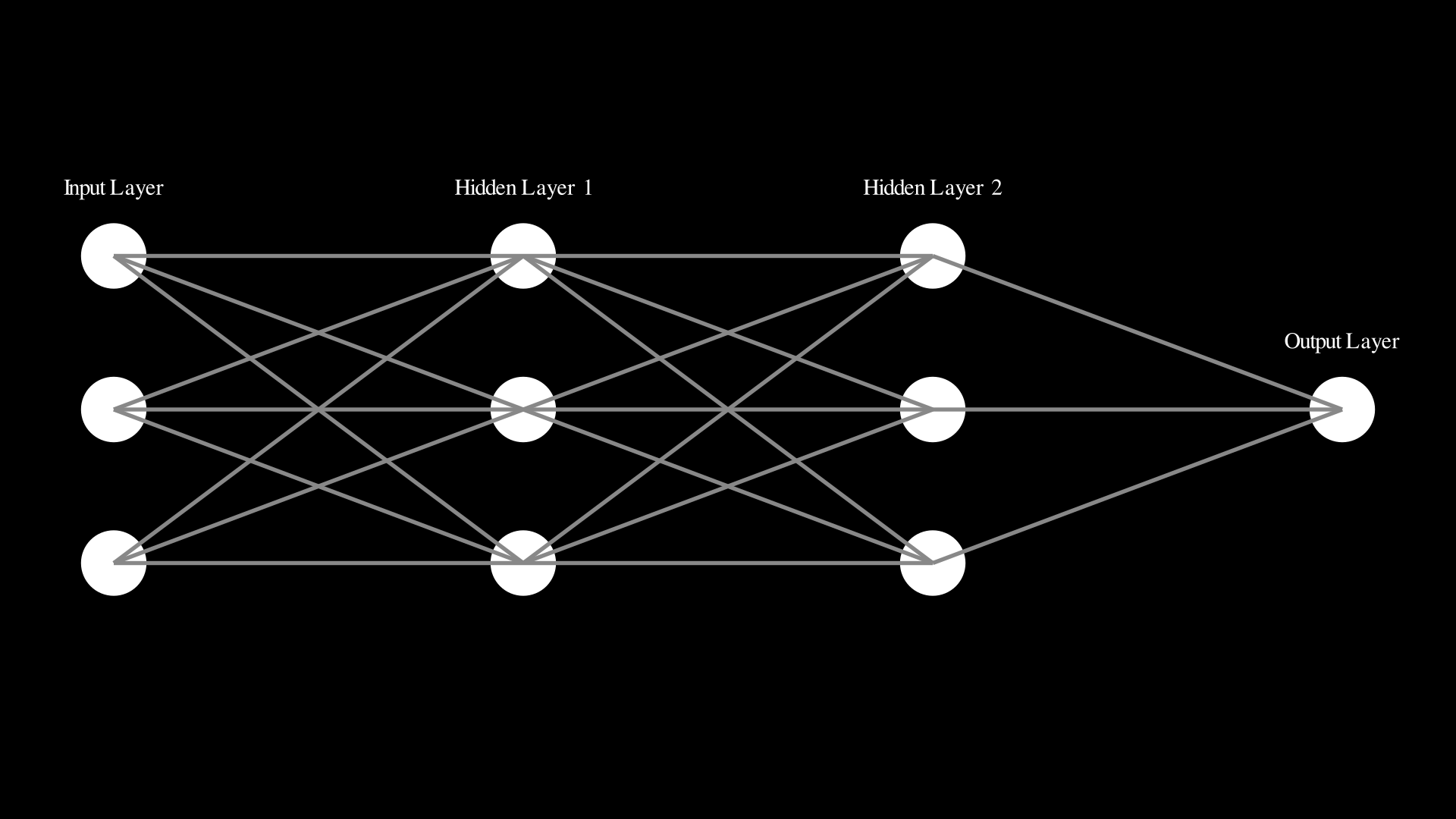
The architecture of neural networks
It helps to visualize the architecture of neural networks in a more intuitive way.

now lets explain some terminology that lets us name differnet part of a network.
- Input layer: The leftmost layer in this network is called the input layer, because it receives the input data from the outside world.
- Output layer: The rightmost layer in this network is called the output layer, because it produces the output data.
- Hidden layer: Since the neurons in this layer are neither inputs nor outputs. The term “hidden” perhaps sounds a little mysterious but it really means nothing more than “not an input or an output”. The network above has just a single hidden layer, but some networks have multiple hidden layers.
For our classfication problem we have a 28x28 pixel image, and we want to classify it as a number between 0 and 9. So we will have an 784 input neurons, and 10 output neurons.
To recognize individual digits we will use a three-layer neural network:
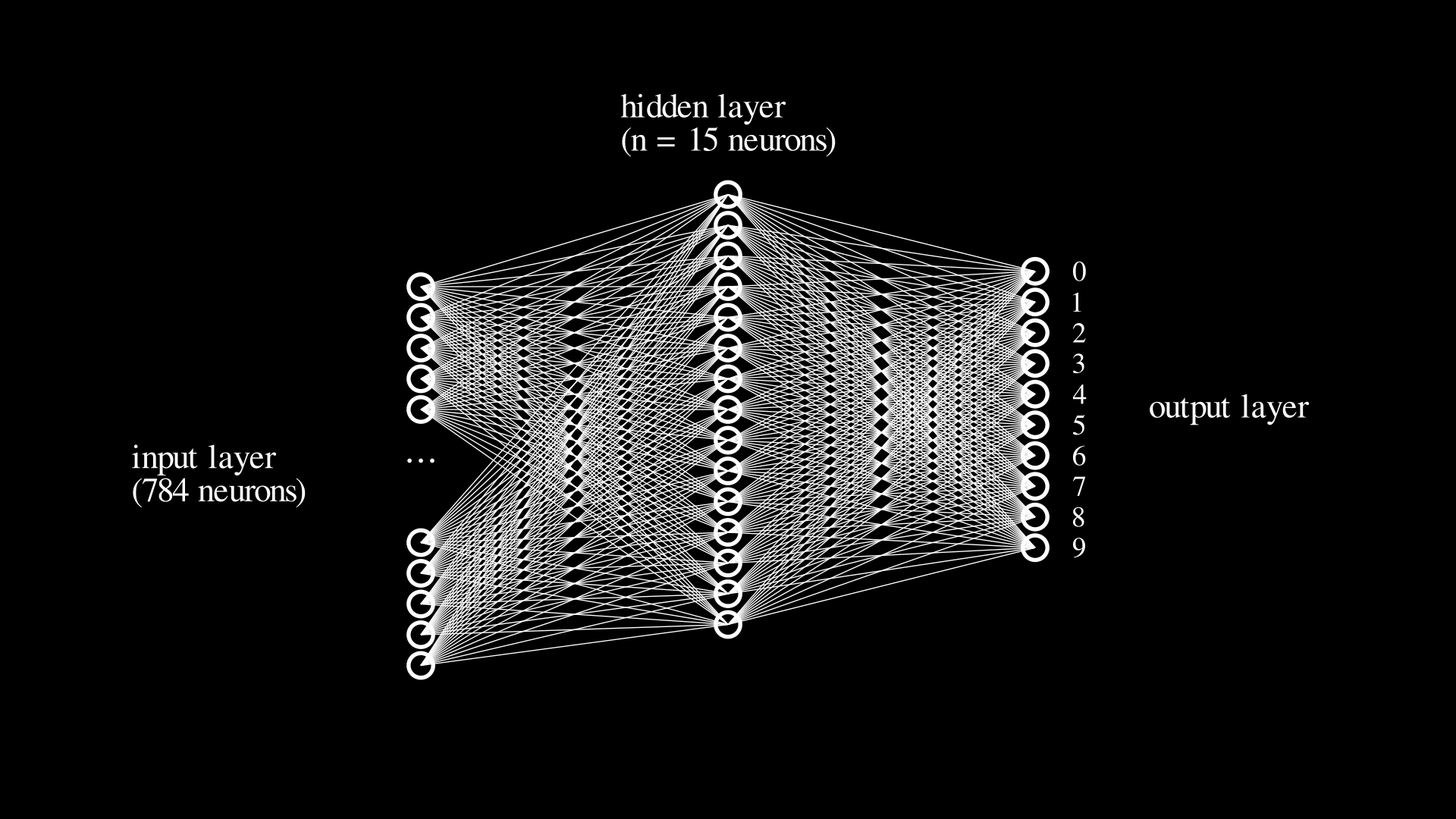
The input layer of the network contains neruons encoding the values of the input pixels.As dicussed above, our training data for the network will consist of many 28 by 28 pixel images of handwritten digits. The input pixels are greyscale, so each pixel is represented by a value between 0.0 representing white and 1.0 representing black.
The second layer of the network is a hidden layer. We denote the number of neurons in this layer by $n$, and we’ll experiment with different values of $n$.
The output layer of the network contains 10 neurons. Each neuron corresponds to one of the 10 possible classes. If the first neuron in the output layer is active, then the network predicts that the input image is a 0. If the second neuron is active, then the network predicts that the input image is a 1, and so on.
To understand what the network is doing. Let’s consider the first output neuron , the one that’s trying to decide whether or not the digit is a 0. It dose this by weighing up the valuse from the hidden layer of neurons.
Lets see this this digit 0:

layer detects whether or not an image like this is a 0. by weighing input pixels which overlap with the image,
let’s suppose that the first, second, third, and fourth neurons in the hidden layer detect whether or not following images are presnet:


As you may have guessed, these four images together make up the 0 image that we are saw earlier. So if all four of these hidden neurons are firing then we can conclude that the digit is a 0.

Look to this gif, the network is trying to detect whether or not the digit is a 0. by weighing input pixels,the hidden layer contains 30 neurons, and an number of those neurons are firing to the 0 neuron in the output layer.
Learning algorithm
We’ll use the gradient descent algorithm to train the network. The gradient descent algorithm is a simple optimization algorithm that is used to find the minimum of a function. In this case we need to chose the function that we want to minimize in way to let us find the weights and biases so that the output from the network is as close as possible to the desired output.
The function that we want to minimize is the cost function. The cost function is a measure of how well the network is doing at classifying the input images. The cost function is defined as the sum of the squared differences between the actual output of the network and the desired:
$$ \begin{align} C(w,b) = \frac{1}{2n}\sum_{i=1}^{}(y_i - \hat{y}_i)^2 \end{align} $$
Here, $n$ is the number of training examples, $y_i$ is the desired output for the $i$ th training example, and $\hat{y}_i$ is the actual output of the network for the $i$ th training example. Here $w$ denotes the collection of all weights in the network, and $b$ denotes the collection of all biases in the network. We’ll call $C$ the quadratic cost function; it’s also sometimes known as the mean squared error or the mean squared loss or just MSE.
Okey. let’s suppose we’re trying to minimize the cost function, $C(w,b)$. What we’d like is to find where $C$ achieves its global minimum. Let’s this about what happens if we change the weights and biases a little bit and see how the cost function changes. Calculus tells us that $C$ changes as follows: $$ \begin{align} ∆C \approx \frac{dC}{dw}∆w + \frac{dC}{db}∆b \end{align} $$
We’re going to find a way of chossing $∆w$ and $∆b$ so that $∆C$ is as small as possible. To figure out how to do that it helps to define $∆w,∆b$ as $∆v$ to be the vector of changes in the weights and biases. $∆v \equiv (∆w,∆b)^T $, where the $T$ denotes the transpose of a vector, turning row vectors into column vectors. We’ll also define the $gradient$ of $C$ to be the vector of partial derivatives of $C$ with respect to the weights and biases. We’ll denote the gradient as $∇C$. $$ \begin{align} ∇C \equiv (\frac{dC}{dw},\frac{dC}{db})^T \end{align} $$ $∇$ is the gradient operator, is just a piece of notation that tells us the $∇C$ is a gradient vector of $C$.
Now with these definitions we can write the expression for $∆C$ as follows: $$ \begin{align} ∆C \approx ∇C^T ∆v \end{align} $$
Now what is really interesting in this equation (12) is that we can choose $∆v$ so as to make $∆C$ as small as possible. In particular, suppose we choose
$$
\begin{align}
∆v = −η∇C
\end{align}
$$
where $\eta$ is a small positive number called the learning rate. Then we have $∆C ≈ −η∇C ⋅ ∇C = −η∥∇C∥^2$. Because $∥∇C∥^2$ is always nonnegative, this means that $∆C$ is always nonpositive, and so it’s always decreasing. This is a nice property that we’ll want to have in our optimization algorithm.
Let us see how this works in simple example. Suppose we have a $C(x) = x^2$ function, this a simple function our goal is to minimize it. First we calculate the gradient of $C(x)$, which is $∇C(x) = 2x$. Second is step update, the equation of the gradient descent is: $$ \begin{align} x_{new} = x_{old} − η∇C \end{align} $$
Now let us assume that the $learning rate$ $η = 0.1$ and the initial value of $x = 3$, gradient when $x=3$ is $2(3) = 6 = ∇C $. The the step update is: $$ \begin{align} x_{new} = 3 − 0.1(6) = 3 − 0.6 = 2.4 \end{align} $$ Calulate the $cost function$:
before update. $$ \begin{align} C(x) = 3^2 = 9 \end{align} $$ After update. $$ \begin{align} C(x) = 2.4^2 = 5.76 \end{align} $$
The change in cost function is $∆C = C(x_{new}) - C(x) = -3.24$. Notice that the change in cost function is negative, which means that the cost function has decreased. This is what we want, because we want to minimize the cost function.
When we compare that with the theoretical equation, $∆C ≈ −η∥∇C∥^2$, we will get $∥∇C∥^2 = (6)^2 = 36$. And then $∆C ≈ −0.1(36) = -3.6$. This is the same as the change in cost function, which is $∆C = -3.24$. So the step update is correct.